Expectation Maximization

In this post we shall explore expectation maximization, a mathematical tool used in many generative AI algorithms, in detail. Expectation maximization is a means to calculate the maximum likelihood estimate in presence of latent variables.

1. Background

In this section we cover the necessry definitions and notations to understand the expecation maximization algorithm:

1.1 Definitions

Let \(X= \{x^{(1)}, x^{(2)}, ....x^{(3)} \}\) be samples taken from a distribution model parameterized by \(\Theta\) as part of an experiment:

Probability: Chance of occurance of an event.
Probability distribution: A mathematical function that gives probabilities of all the possible outcomes of an experiment, written as \(P (x^{(i)} \mid \Theta )\). The sum of probabilities of all outcomes must sum to 1 .
Likelihood: If the paramter of a distribution model are represented as \(\Theta\) , then the likehood function is the joint probability of all the observed data points as a function of \(\Theta\) i.e. it outputs the likeliness of different values of the parameter \(\Theta\) to model the distribution from which the observed data could be sampled, written as \(L(\Theta \mid X)\).
Maximum Liklihood: Mechanism to find the value of \(\Theta\) that maximizes the likelihood function given \(X\).
Latent variables: Assume that each \(x^{(i)}\) is dependent on another random variable \(Z^{(i)} = \{ z_1^{(i)}, z_2^{(i)},...z_k^{(i)} \}\) that is not observed. Such a variable is called hidden or latent variable. \(Z\) is called latent variable because it is not observed. Each observation \(x^{(i)} \in X\) is dependent, with some probability on all possible \(K\) values of \(Z\), called the posterior.
Evidence: The probability distribution of X , denoted as \(P(X)\) i.e. the probability ditribution of observed data.
Posterior: The probability distribution of latent variables Z given \(x^{(i)} \in X\), denoted as \(P(Z \mid x^{(i)})\) .
Prior: The probability distribution of latent variables known from prior experience, denoted as \(P(Z)\)
Model: A computational framework that maximizes the joint probability of variables X and Z parameterized by \(\Theta\), denoted as \(\displaystyle \sum_i^N \sum_j^K P(x^{(i)},z_j^{(i)}; \Theta)\). This , can be evaluated as: \(P(X \mid Z,\Theta) * P(Z)\), using Baye’s rule.
Cordinate descent: is a an iterative optimization algorithm. Each iteration involves two steps. In the first step the algorithm optimizes the objective by updating only a subset of parameters influencing the objective, while keeping the remaining parameters fixed. In the next step, it fixes the values of the parameter subset changed in first step and optimizes the objective by changing the remaining ones.

1.2 Jensen’s Inequality:

\(E[f(x)] \ge f( E(x))\) , when \(f\) is convex
IF f is stricly convex AND \(E[f(X)] = f( E(X) )\) THEN
\(X = E(X)\) with probability 1 i.e. the value of X is a constant.

2. Expectation Maximization (EM)

If we are tasked with creating a computational model which maximizes the probability of observed data \(X=\{x^{(1)}, x^{(2)}, ....x^{(n)} \}\) each of which are dependent latent variables \(Z=\{z_1, z_2, .... z_k\}\) , it is not possible to get a closed form equation to maximize the liklihood function of the joint probability of \(X\) and \(Z\) . Expectation maximization, tries instead to obtain the maximum liklihood of the observed data by indirectly accounting for Z using a co-ordinate descent approach.

2.1 Derivation of EM Algoritm

The objective of EM algorithn is to maximize the log likelihood of the observed data in presence of latent variables:

Log Likelihood function: \(\displaystyle L(\Theta \mid X ) = \sum_{i=1}^N log (P(x^{(i)}; \Theta))\)
The above equation can be modified to introduce \(Z\): \(\displaystyle L(\Theta \mid X ) = \sum_{i=1}^N \sum_{j=1}^K log ( P(x^{(i)},z_j^{(i)}; \Theta ) )\)
Let us assume there is a distribution \(Q\) from which \(Z\) is sampled for each \(x_i\). We multiply and divide the above expression by \(Q(z_j)\): \(\displaystyle L(\Theta \mid X ) =\sum_{i=1}^N \sum_{j=1}^K log \frac{ Q(z_j) * P(x^{(i)},z_j^{(i)}; \Theta ) }{ Q(z_j^{(i)}) }\)
By definition of expectation: \(\displaystyle L(\Theta \mid X ) = \sum_{i=1}^N log ( E_{z \sim Q(Z^{(i)})}\frac{P(x^{(i)},z, \Theta ) }{ Q(z) })\)
Since \(log\) is a concave function,using Jenson’s inequaltity: \(\displaystyle L(\Theta \mid X ) \ge \sum_{i=1}^N E_{z \sim Q(Z^{(i)})}log( \frac{P(x^{(i)},z, \Theta ) }{ Q(z) })\)

This expression is termed as \(ELBO(X, Q, \Theta )\) or the Evidence Lower Bound and based on the above derivation, it is clear that \(L(\Theta \mid X )\) is always greater than this value.

2.2 Deriving Q

Jenson’s inequality states that ELBO will be exactly equal to \(L(\Theta \mid X )\)

if \(\displaystyle \frac{P(x^{(i)},z, \Theta ) }{ Q(z) } = c\), a constant
This implies: \(\displaystyle Q(z) \propto P(x^{(i)},z, \Theta )\)
Since \(Q\) is a probability distribution \(\sum_z Q(z)=1\). Therefore to convert proportionality to equality, we can normalize the right-hand side: \(Q(z) = \displaystyle \frac{P(x^{(i)},z, \Theta )}{\sum_z P(x^{(i)},z, \Theta )}\)
Q(z) = \(\displaystyle \frac{P(x^{(i)},z, \Theta )}{P(x^{(i)},\Theta )}\)
Q(z) = \(\displaystyle P(z \mid x^{(i)})\)

This implies that the best likelihood value can be achieved for given parameters \(\Theta\) if we can minimize the KL-Divergence between \(Q(Z^{(i)})\) and \(P(Z^{(i)} \mid x^{(i)})\)

2.3 The EM Algorithm

Using the derivations above, the EM Algorithm can be framed as follows:

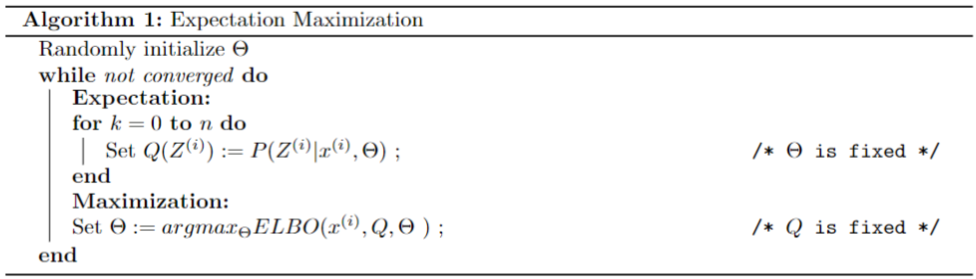
The Expectation step calculates the value of \(Q(z)=P(z \mid x^{(i)})\), the value at which ELBO is exactly equal to \(L(\Theta \mid X )\) for a specific value of \(\Theta\).
The Maximization step, calculates the new value of \(\Theta\), that would maximize the or the value of \(ELBO(X, Q, \Theta )\) with the value of \(Q\) calculated in the expectation step held constant.
These two steps performed iteratively converges the parameters \(\Theta\) towards values that maximizes the value of \(L(\Theta \mid X )\).

2.4 Calculating Q

Calculating value of \(Q(z)\) in the EM algorithm requires calculating \(P(z \mid x^{(i)})\). There are different ways to do that:

Analytically, by using Baye’s theorm.However, for complex models the posterior cannot be calculated analytically
Emperically, using MCMC (Markov Chain Monte Carlo) techniques like Gibbs Sampling to approximate it’s value.

Lastly, an alternative to using MCMC to approximate the posterior of a complex model, we can use mean-field variational inference, a topic discussed in the next post.

3. Example: Univariate Gaussian Mixture Model

In this section, we see will see how expectation maximization algorithm is applied to Gaussian Mixture Models. The generic expectation maximization algorithm derived above places no restriction on underlying distribution type that generates the data. Gaussian Mixture Models model data that is derived from multiple gaussian distributions. The latent variable, is a categorical variable that ditermines the softmax ( probability distribution) of gaussian distributions an observation is derived from.

3.1 Given

As a first step to model any data we identify what information is available to us.

Evidence = \(x^{(i)}\), for i=1,2,…, \(N\)
The fact that the observations are depedent on a latent variable = \(Z\), which is categorical
Number of different values the latent variable can take:\(K\)

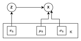
3.2 Model

Next, we decide that we shall use gaussian distribution to model the latent variable.

\(Z^{(i)}\) = multinomial(\(\pi\))
and \(P(x^{(i)} \mid Z^{(i)}) = \mathcal{N}(\mu_{Z^{(i)}},\sigma^{2}_{Z^{(i)}})\)

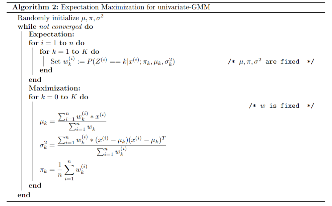
3.3. Algorithm

To derive the algorithm to fit data into a gausssian mixture model, we refer the general expectation maximization algorithm:

\(\Theta=\pi,\mu,\sigma^{2}\) , where each parameter is a K-dimensional vector.
Expectation:
- \[\displaystyle w_k^{(i)} = Q_k * P(z_k^{(i)} \mid x^{(i)})=\frac{P(x^{(i)} \mid z_k^{(i)}) *P(z_k^{(i)})}{P(x^{(i)})} = \displaystyle \frac{P(x^{(i)} \mid z_k^{(i)}) *P(z_k^{(i)})}{\sum_k P(x^{(i)} \mid z_k^{(i)})*P(z_k^{(i)})}\]
- \(P(x^{(i)} \mid z_k^{(i)})\) can be replaced with \(\mathcal{N}(\mu_{z_k^{(i)}},\sigma^{2}_{Z^{(i)}})\)
- \(P(z_k^{(i)})\) with \(\pi\)
Maximization
- in \(ELBO(X, Q, \Theta )\) \(P(x^{(i)},z_k^{(i)}, \mu_k,\sigma_k )\) is replaced with \(P(x^{(i)} \mid z_k^{(i)}) * \pi\)
- The result in then partially differentiated for each parameter \(\mu_k,\sigma_k,\pi_k\) and equated to zero the find out the value of the parameters, resulting in the following algorithm.

Refer to this link for a very good example of implementation of gaussian mixture model in python.

4. References

Written on October 1, 2023